SEMANTIC SIMILARITY AND TOXICITY DETECTION IN QUORA QUESTIONS
INTRODUCTION
300 million monthly active users use Quora, a question and answer platform for asking their queries on anything piquing their curiosity and also publish their unique experiences and knowledge in the answers. Such a tremendous platform used by seekers, writers, and viewers faces the issue of duplicate or similar meaning questions. This decreases the proliferation of good content and increases the effort of writers. With an increasingly social world, the polarization of content is also an issue to be tackled. Questions disparaging a community or posing a threat to the fabric of society need to be moderated.
PROBLEM DEFINITION
Online Social Networks continue to play an important role as information is regularly uploaded and exchanged. Abuses of such media of communication for various malicious purposes are very common. We need to identify such content and flag it appropriately for creating a safe platform.
Also, Question duplication is a major problem in any public discussion forum. Fragmentation of answers across various versions of the same question results in a lack of a sensible search, answer fatigue, segregation of information, and the paucity of response to the questioners. The duplicate questions can be detected using Machine Learning and Natural Language Processing.
Our aim is to solve 2 problems:
- When 2 questions are given as an input, we find if they are similar or not?
- When 1 question is given, we classify if the question is appropriate or not? and the output if there are any similar questions to the given on in the dataset.
These problems are not related, but are of major concern to a question-answer platform like Quora, Piazza etc. So we build different models to tackle these problems. Additionally, we propose a unique solution of displaying similar questions using clustering.
PROPOSED METHODS
For question-pair input
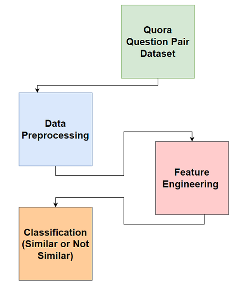
For single question input
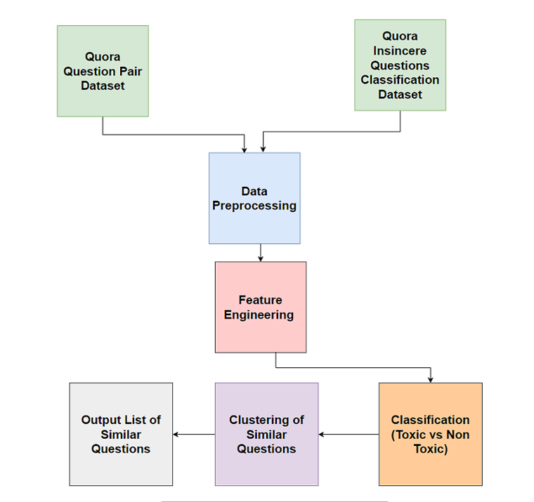
We identify the two datasets we will use to solve this challenge. They are released by Quora.
Datasets:
- Quora Question Pairs Dataset for finding the similarity between questions.
- Quora Insincere Questions Classification Dataset for detecting any objectionable/toxic content in the questions.
To convert the initial corpus of text to a standard form, we perform the below data preprocessing steps.
Data Pre-processing:
- Stop-word, punctuation removal
- Stemming/Lemmatization
- Lower-case conversion
The next step is to generate embeddings from the cleaned data. We will compare the below methods that work best for our model.
Feature Engineering:
- TF-IDF
- Word2Vec/Glove neural network
- Elmo-embeddings
- Latent Semantic Indexing
Proceeding to perform unsupervised learning to cluster similar questions.
Clustering of similar questions:
- K-means
- DBSCAN
- Spectral clustering
The machine learning methods can provide us good results on the classification of content as toxic or not:
- Random Forest
- SVM
State-of-the-art Deep learning methods will be trained on the datasets and the results of toxicity classification and similar question clustering will be benchmarked.
- LSTM
- BERT - Can generate own embeddings too.
- Gated Recurrent Unit
DATASET COLLECTION
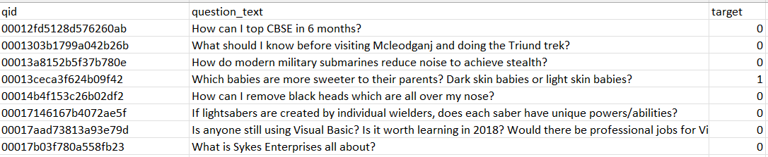
For the task of predicting if a question is insincere or toxic in the Quora Platform, the dataset Quora Insincere Questions Classification is used. This dataset was released by Quora on the Kaggle platform as a challenge. For each question id in the test set, users must predict whether the corresponding question_text is insincere (1) or not (0).
A few rows of the dataset are displayed below. We have three columns - one indicating the question ID, another is the text of the sentence and the other is the target which is 0/1 depending upon the question being sincere or not.
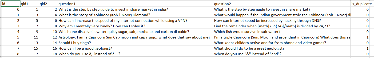
The Quora Question Pairs Dataset was released as a Kaggle Challenge by Quora in 2016. The challenge aimed to find the minimum logloss on the test dataset on the probability predictions that the questions are duplicates. The motivation behind the challenge was to improve the usability and efficiency of the Quora platform and make it easier for users and writers to avoid redundant questions.
Sample rows of the dataset look like below. This dataset has 6 columns namely - ID, QID 1 which is the unique ID of the question 1, QID 2 which is the unique ID of the question 2, question 1 and question 2 are text strings and is_duplicate indicating if the questions are duplicate or not.
The two datasets are explored in detail in the following sections.
METHODS
Quora Insincere Questions Classification Datasets
Exploratory Data Analysis
We use the Quora Dataset released in a Kaggle challenge.
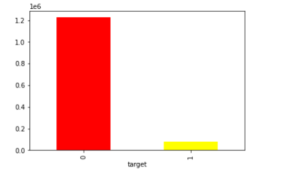
The dataset contains 1306122 samples each with three features - [‘qid’, ‘question_text’, ‘target’] The question text is a question asked on Quora.Target = 1 denotes an insincere question while target=0 denotes a sincere question.
We visualize the count of the two classes and observe a huge imbalance skewed towards sincere classes.
Bar plot of the distribution
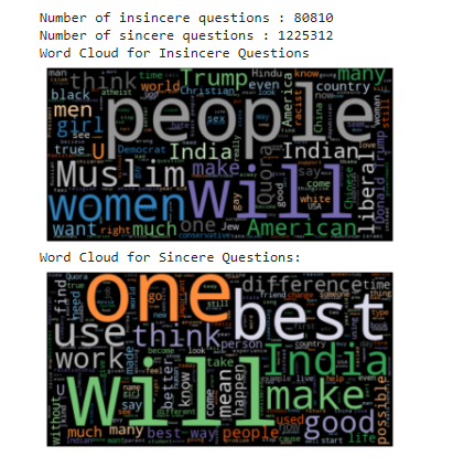
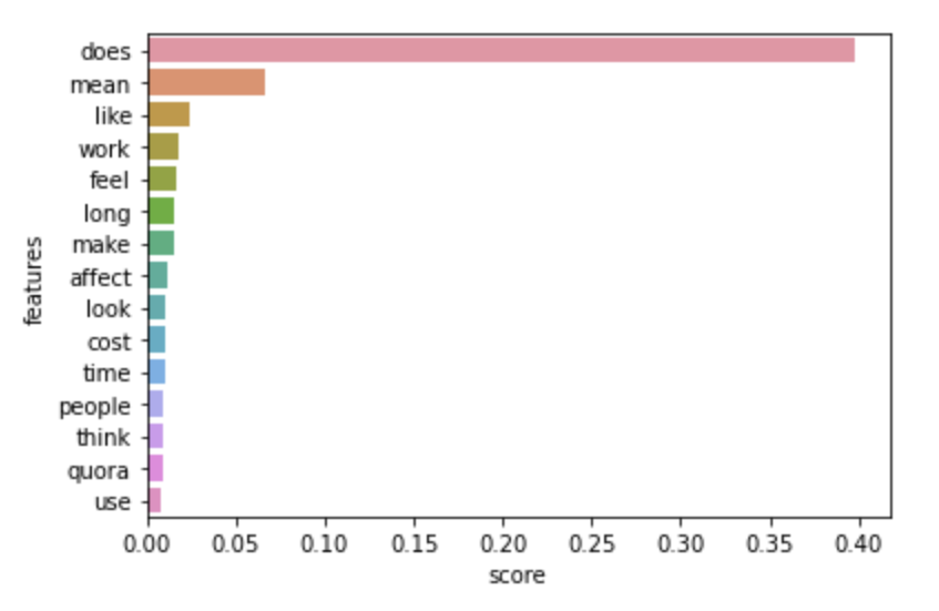
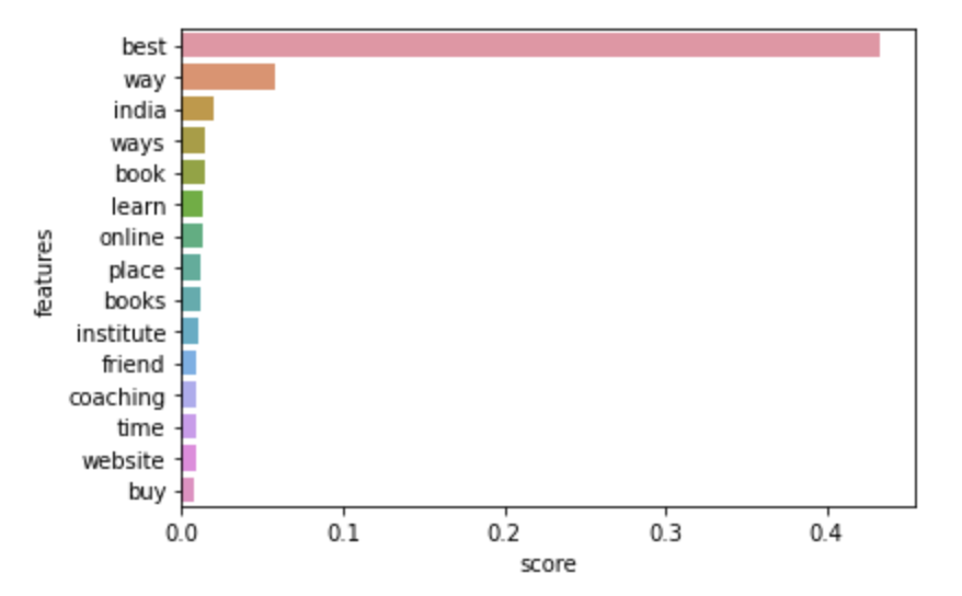
We also plot wordclouds for sincere and insincere questions to get an idea of the words most frequent in the two classes.
Data Pre-processing:
-
Stop-word/punctuation removal: Before we begin working on our data, as traditionally carried out in most NLP practices, we remove stop words and remove punctuation in the questions on both datasets. These words unnecessarily occupy extra memory in the database and contribute to the processing time. For this purpose, we use NLTK in python.
-
Stemming & Lemmatization: Post the removal of stopwords, we have also carried out stemming and lemmatization using NLTK so that only the essence of each word is retained. Lemmatization is a more meaningful simplification than stemming since it reduces each word semantically, based on its meaning. Stemming does a more ‘raw’ reduction into its corresponding root but is computationally less expensive. We have used both the simplifications as part of our analysis. We used snow-ball stemming.
-
Lower-case conversion: All the words are also converted to lower-case to avoid the possibility of the algorithms mistaking two same words with different cases of alphabets as two distinct words. It is a very simple but essential step and greatly helps in increasing the consistency of the output.
Feature Engineering
-
Count Vectorizer (One-Hot Encoding): One of the most basic ways to represent text data numerically. The concept behind Count Vectorizer is to create a vocabulary vector and check if text data features that vocab word. If it features we add one n that dimension and increase the count every time we encounter a word.
-
TF-IDF: We use TF-IDF as a feature engineering step to convert the question-text into a vector to feed into the algorithms. It is a version of the bag-of-words method for vectorization, and we preferred this method since some priority is given to the ‘importance’ of the word.
It is calculated as a product of Term-Frequency (TF) and Inverse-Document-Frequency (IDF).
Term Frequency (TF) can be calculated as the ratio of a word’s occurrence in a question to the total number of question words. But with term frequency, the importance of a word cannot be measured, but just gives weightage to how ‘frequent’ a word is.
Inverse Document Frequency (IDF) is measured as the natural log of the ratio of (total number of questions in the entire database)/number of questions containing the word
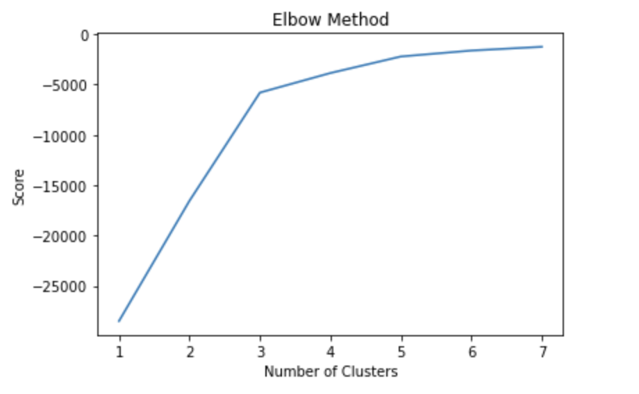
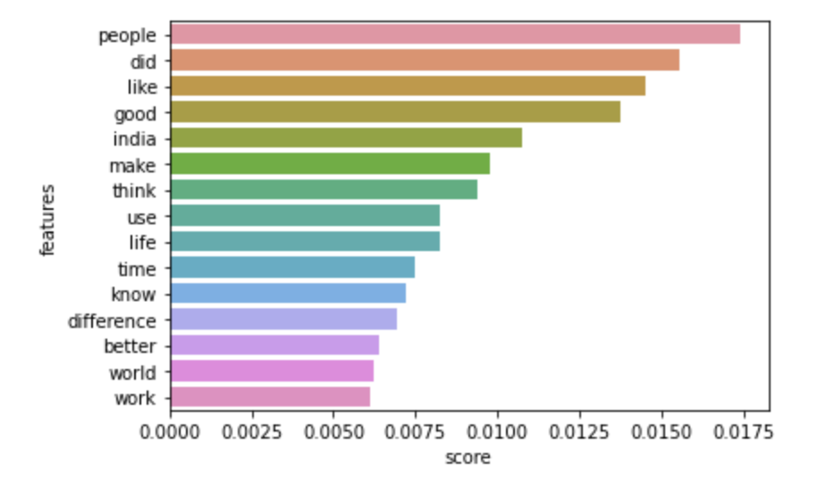
- Clustering:
We wanted to get some quick insights from the data and it was too large to interpret it manually. Therefore, we decided to go for a simple k-means clustering to quickly mine information.
So, we vectorized the data using TF-IDF to retain the semantic significance while feeding the data to k-means.
We obtained 3-clusters by using the elbow method, as can be seen below. The most frequent words according to the cluster are also plotted below and is useful in giving us cues about the distribution of words and data among classes.
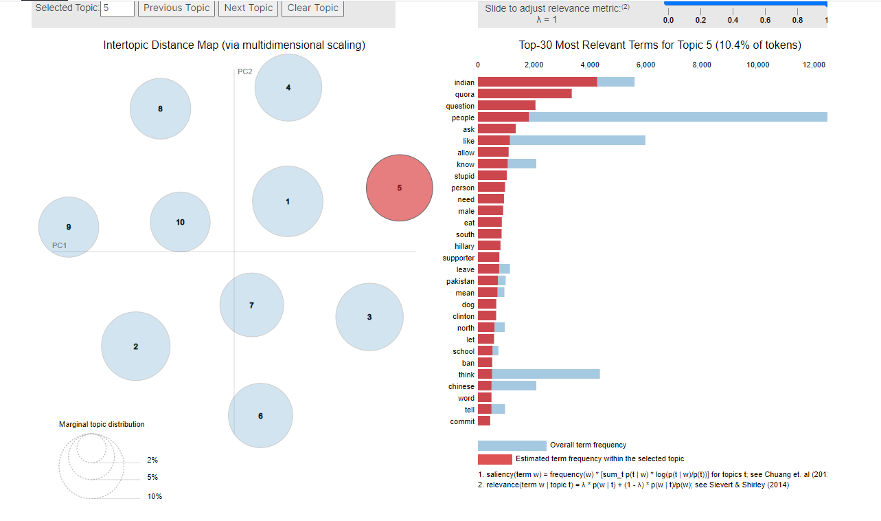
Latent Dirichlet Allocation / LDA:
Latent Dirichlet Allocation is a probabilistic topic modeling technique used to uncover the thematic structures in a text corpus. This is performed on the Dataset for each of the sincere and insincere classes to get an idea of how frequently certain topics appear in each of them. The “topics” generated are clusters of similar words in a document which are determined statistically.
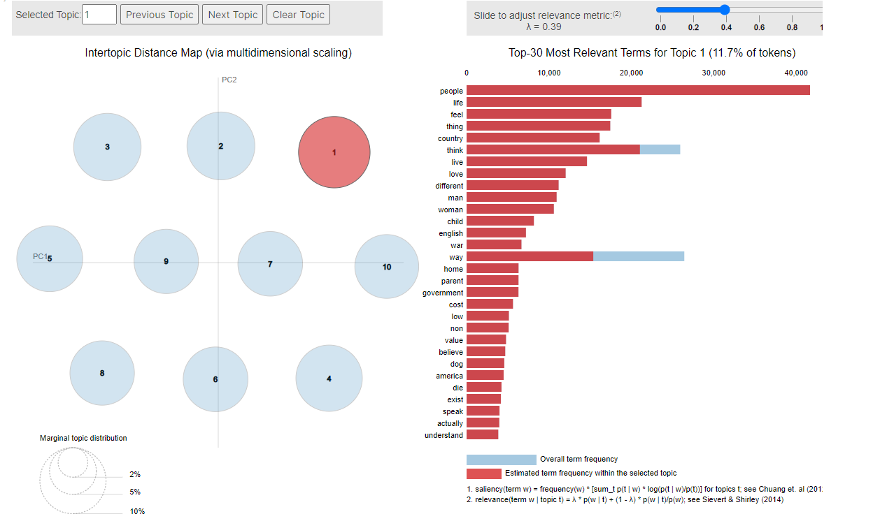
We used pyLDAvis to visualize the trained LDA model and were able to observe the following results. Insincere questions generally have topics of political leaders, racism, and hate.
LDA Insincere Questions
LDA Sincere Questions
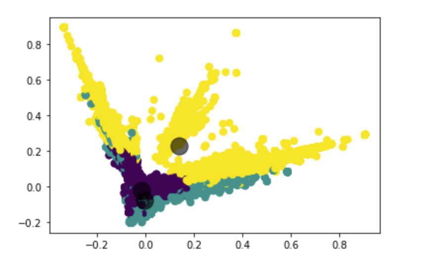
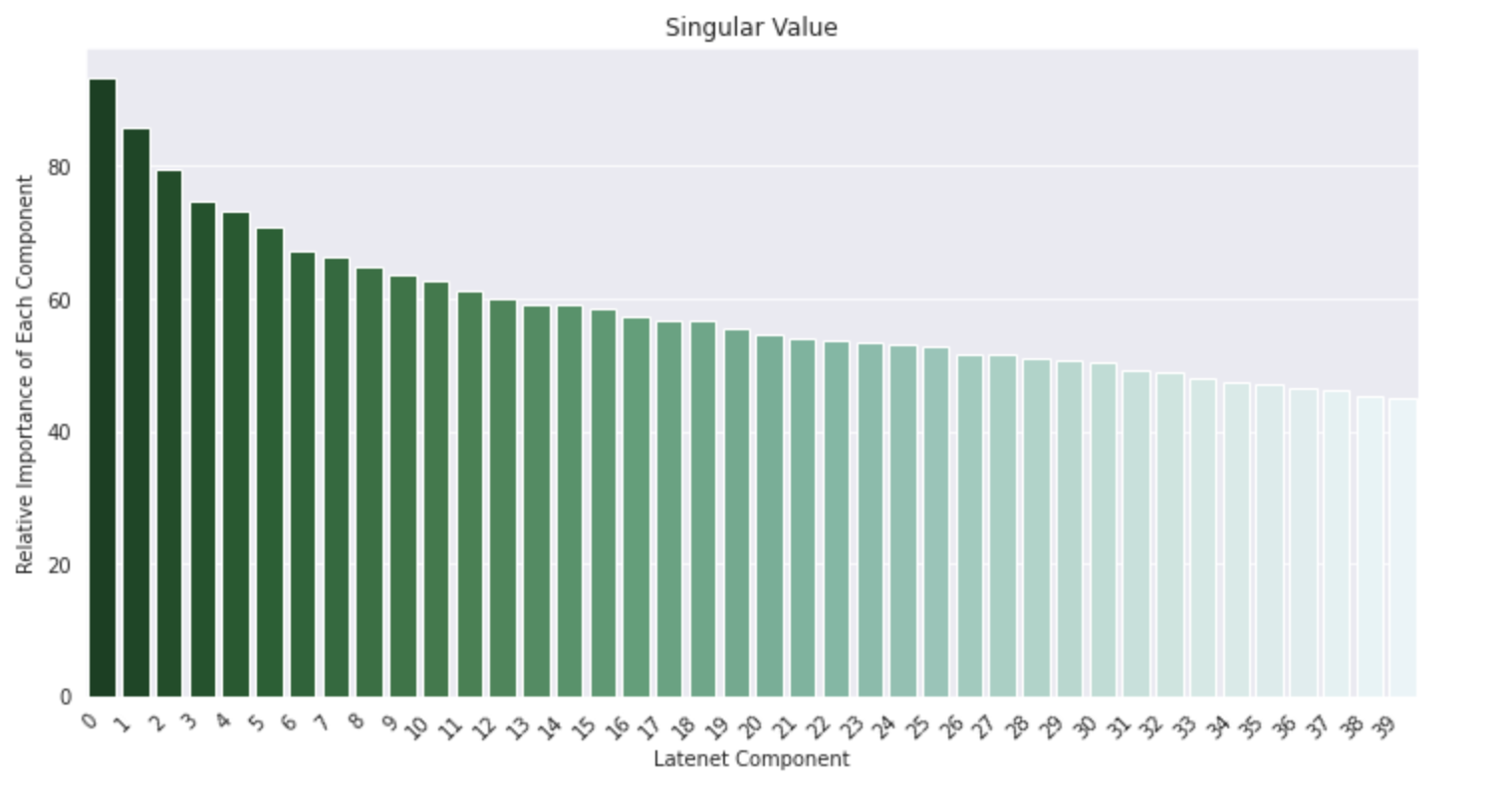
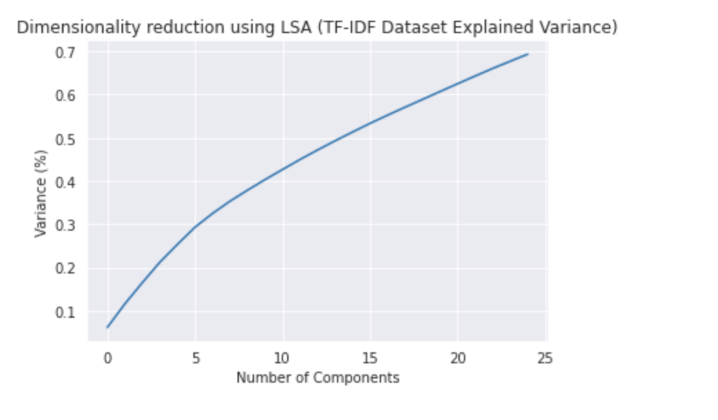
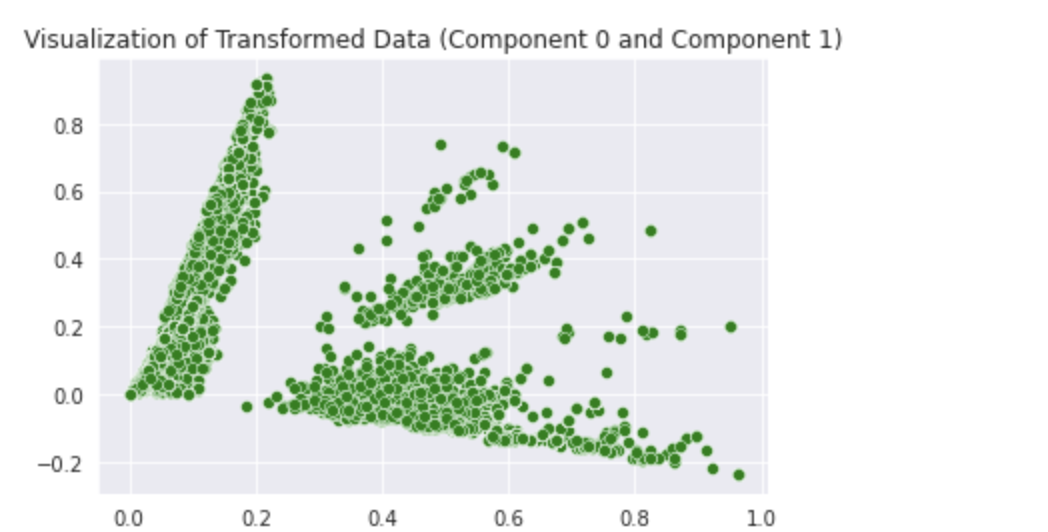
Latent Semantic Analysis / LSA :
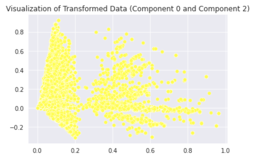
LSA is an unsupervised learning technique. In the Quora Insincere Classification dataset, we use LSA with TF-IDF. Although LSA is an unsupervised technique often used to find patterns in unlabeled data, we’re using it here to reduce the dimensions of labeled data before feeding it into a model. For now, we visualize our LSA-based transformed data. For purpose of Visualization, we fit our LSA object which is Truncated SVD in sklearn to train data and specify 25 components.
Our Visualization will take place in 3 steps:
- Singular Value Visulization:
- TF-IDF Dataset Explained Variance
- Visualizations of the Transformed Data
We now move on to supervised learning methods for the prediction task.
Supervised Learning Methods
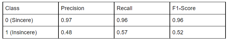
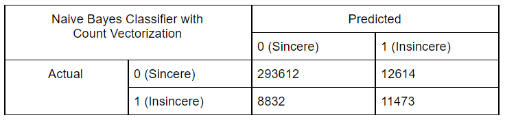
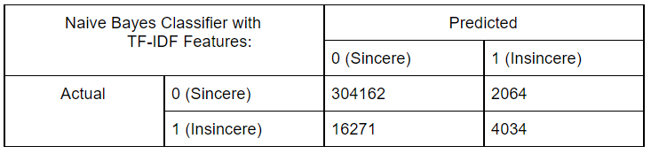
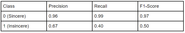
Naive Bayes Classifier:
Naive Bayes Classifier is a Supervised Machine Learning algorithm based on Bayes Theorem. It is a probabilistic model that assumes strong independence between attributes. It is easy to build and particularly useful for large datasets as the computation time is less. Hence, we started off with this model.
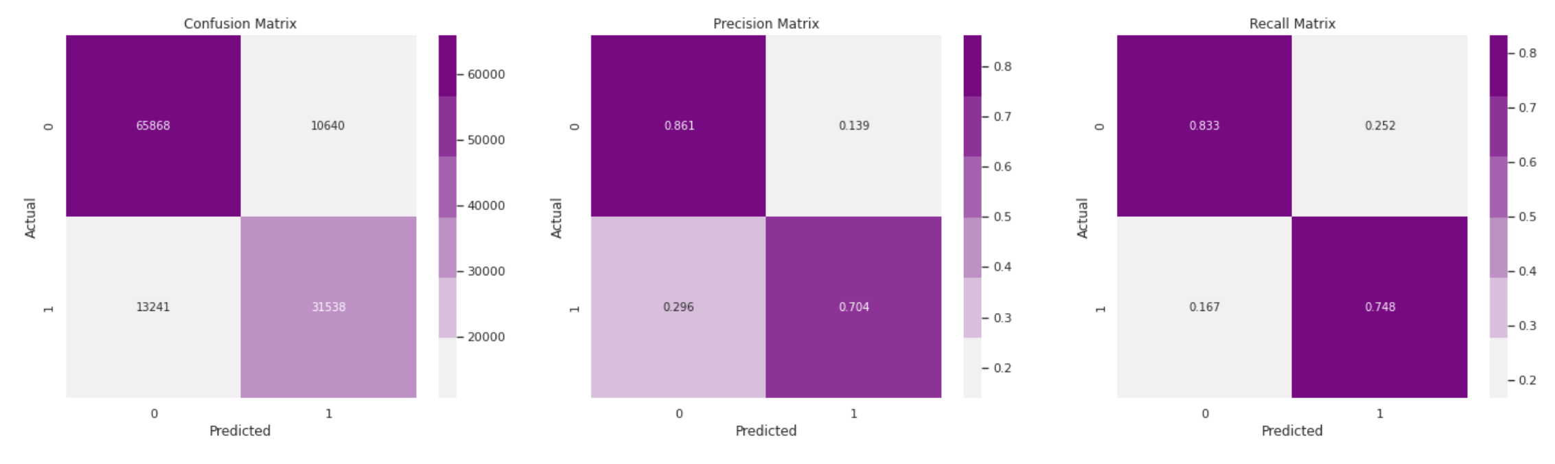
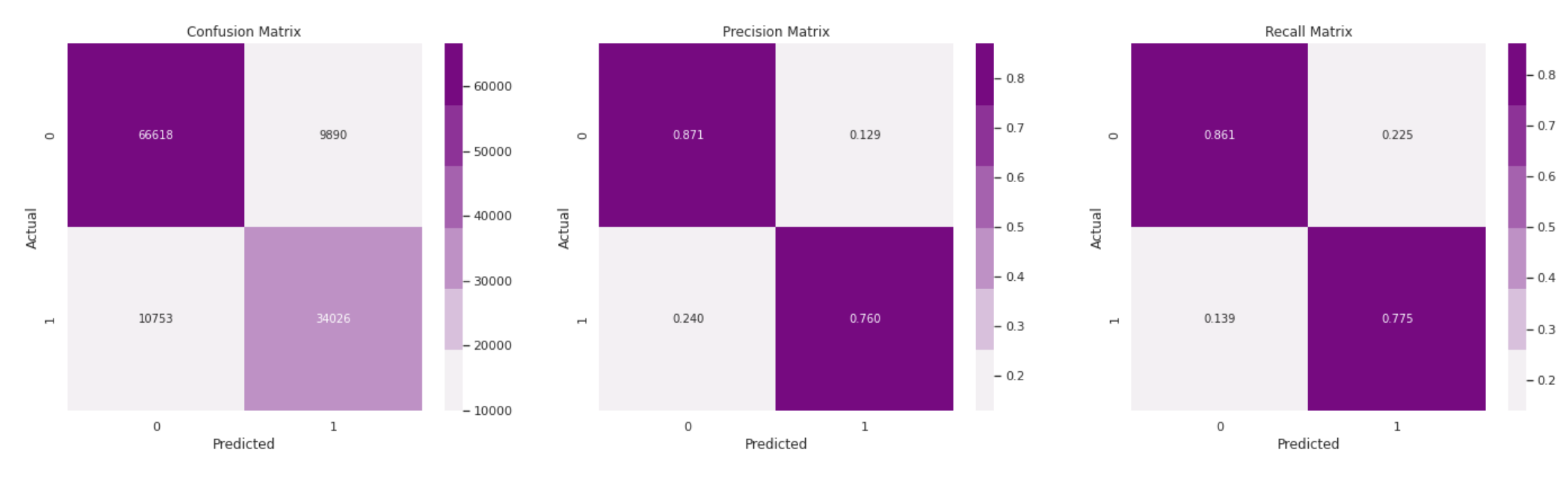
Results:
-
Using Count Vectorization Features:
-
Using TF-IDF Features:
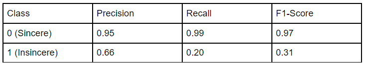
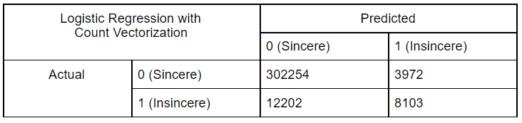
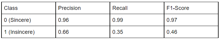
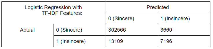
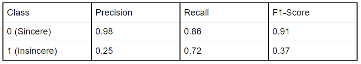
Logistic Regression:
Logistics Regression, also known as the logit model is commonly used for binary classification. The dependent target variable is categorical like Sincere text or Insincere text in our use case. It fits a line to the data separating data points of one class from the other. It estimates the probability of a data point belonging to a class by understanding the relationship between the dependent target variable and independent features.
Results:
-
Using Count Vectorization Features:
-
Using TF-IDF Features:
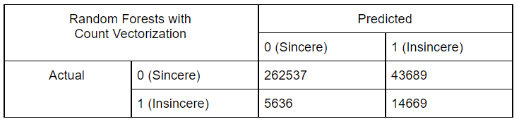
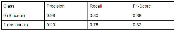
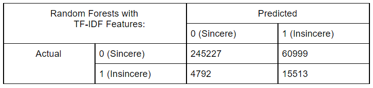
Random Forests:
Random Forests is a supervised ensemble Machine Learning model and is constructed from multiple Decision Trees. It is a bagging algorithm. Random Forests utilize randomness in the features and the data to build each individual tree. The results from all these individual trees are combined to obtain more stable and accurate predictions. This reduces the risk of overfitting.
Results:
-
Using Count Vectorization Features:
-
Using TF-IDF Features:
Note:
- Precision: TP/(TP+FP), We maximise Precision when the cost of reporting False positives is high
- Recall: TP/(TP+FN), We maximise Recall when the cost of missing out on Positives is really high
- f1_score: Harmonic mean of Precision and Recall. F1 score is a better alternative than accuracy when the data used is highly imbalanced like in our dataset.
Deep Learning Architectures:
So far, we have explored Machine Learning algorithms that performed considerably well for this task. Now, we experiment with Deep Learning algorithms to improve performance metric scores. Deep Learning methods have been increasingly gaining popularity over Machine Learning methods as they have the ability to learn latent features from data without explicit rule formulations.
Sequence-to-Sequence Models:
Sequence-to-Sequence models is an umbrella term used for various variations of Recurrent Unit Models. The input is assumed to be sequential data like time-series data, text, and audio. These models are utilized to solve complex problems like Question-Answering, Machine Translation, and Text Summarization to name a few in Natural Language Processing. There are three common kinds of Sequence-to-Sequence Models namely vanilla Recurrent Neural Networks (RNN), Long Short Term Memory (LSTM), and Gated Recurrent Unit (GRU).
RNN:
Recurrent Neural Network is a type of Artificial Neural Network where the outputs from previous states can be fed as inputs to the next state with the help of hidden states. The data is also processed sequentially where each component of the input in a particular timestamp depends upon its previous component in an earlier timestamp. RNN follows a concept known as backpropagation through time where the errors are calculated and accumulated across all the timestamps. The current state in the network cannot be based on any future information. The weights of the Recurrent Neural Network are shared across all the timestamps. RNN sufferers from the vanishing gradient problem. The vanishing gradient problem is where the gradients of the model tend to move towards zero during backpropagation in a deep network with multiple layers.
LSTM:
Long Short Term Memory is a type of Recurrent Neural Network with gates. The gates present in the architecture help the model overcome the vanishing gradient problem. There are It also consists of feedback connections. Each LSTM cell comprises three gates namely input gate, output gate, and forget gate. The forget gate forgets irrelevant information. The input gate adds or updates new information. The output gate passes the updated information. There also exists a cell state in an LSTM cell. As the output of the previous state is passed as input to the current state, the forget gate filters the information given to the LSTM cell. The input gate updates that information with its own new information and the output state passes on this updated information to the next state. All these changes are being made to the cell state in the LSTM cell.
GRU:
Gated Recurrent Unit is similar to LSTM which is also an RNN with gates. It consists of a reset gate and an update gate. The update gate is like a combination of the forget gate and the input gate in LSTM. It filters out information from the previous state and adds new information. The reset determines how much past information to carry forward into the current state and timestamp. It takes the input and the past hidden state information and gives them as inputs to the reset gate where the most relevant information is filtered out. This is fed as input to the update gate where information is erased and added. This results in the new current hidden state which is eventually passed on to the next state. GRU has fewer gates than LSTM. Hence, it is much less complex than LSTM. For certain applications, GRU is believed to converge faster than LSTM. It takes lesser time to train GRU than LSTM as it has fewer parameters than LSTM. Like LSTM, GRU also does not suffer from the vanishing gradient problem.
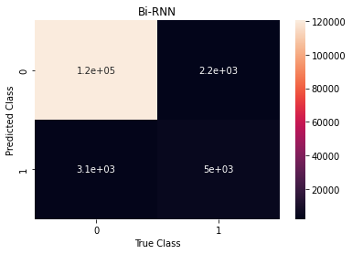
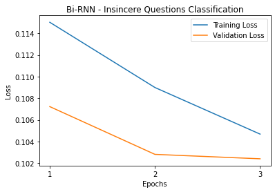
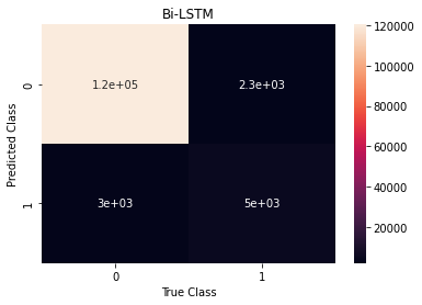
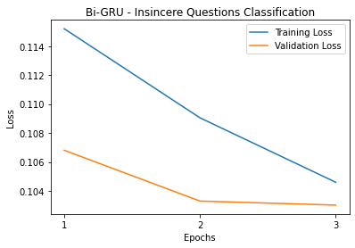
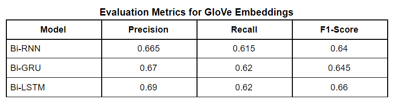
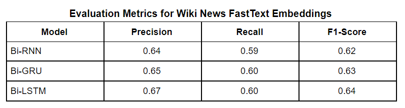
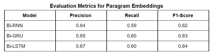
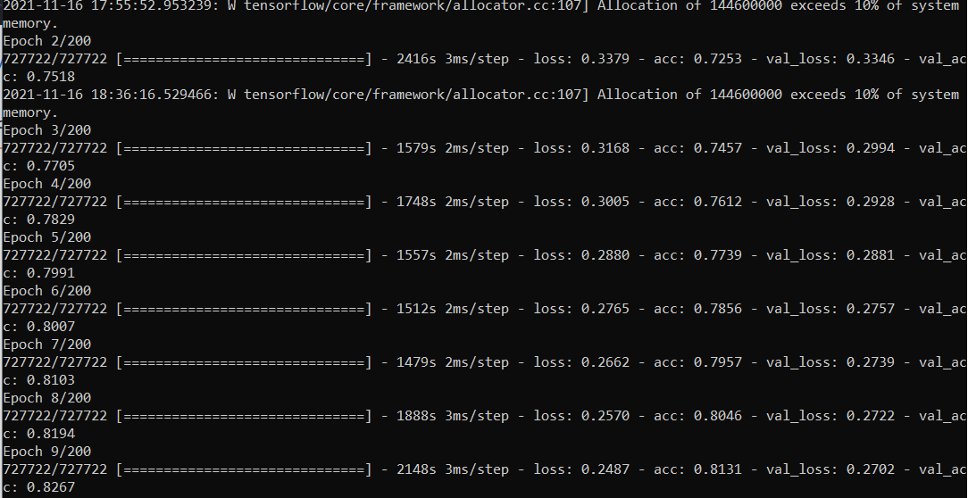
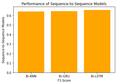
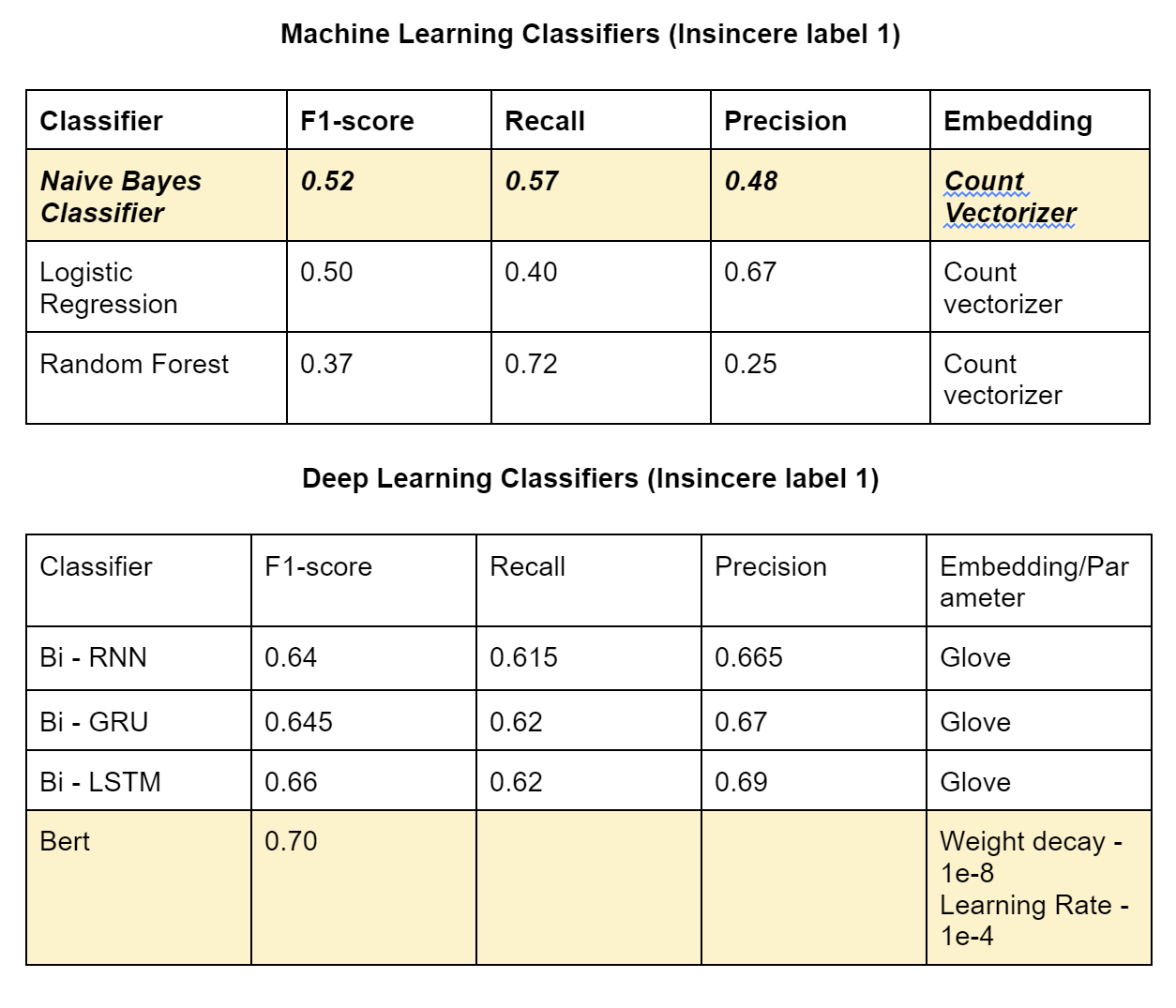
We implemented Bi-directional sequence-to-sequence models. Bi-directional models take the input in the forward direction and backward direction. The backward direction offers a look-ahead into future timestamps. As it is a binary classification problem, we used binary cross-entropy with logits as our loss function. Binary cross-entropy with logits is Binary cross-entropy with a sigmoid layer for thresholding. Among all the optimizers like GD, SGD, and Adam was our choice as it was much faster than other optimizers and we did not face convergence problems with this dataset. A learning rate of 1e-3 was chosen after trying out other learning rates to let the loss of the model decrease gradually but fast enough without much instability in the learning curve. Since the Insincere Questions dataset is imbalanced, F1-Score will be a more appropriate evaluation metric than accuracy. F1-Score takes the distribution of the data into account, unlike accuracy. Accuracy gives more importance to true positives and true negatives whereas F1-Score gives more importance to false positives and false negatives. Bi-RNN, Bi-GRU, and Bi-LSTM attain F1-Scores of 0.64, 0.65, and 0.66 with GloVe respectively. The recall scores for these three models are 0.62, 0.62 respectively. The precision scores for these three models are 0.67, 0.69 respectively. Bi-RNN, Bi-GRU, and Bi-LSTM attain F1-Scores of 0.64, 0.63, and 0.64 with Wiki News FastText embeddings and Paragram embeddings respectively. The recall scores for these three models are 0.60, 0.62 respectively. The precision scores for these three models are 0.65, 0.67 respectively. All the evaluation metric scores for the GloVe are better than the Wiki News FastText and Paragram embeddings individually. This may be due to the global statistics or word co-occurrence incorporation by GloVe.

The results of all models are given below:
Transformer Based Models:
Though sequential models achieve great performance and are well suited to address a range of problems, they have a few drawbacks. Parallelization is inhibited by sequential computation. There is no explicit way to model long-range and short-range dependencies. The distance between positions of entities in data is linear. These issues are solved by Transformers. Transformers are based on the concept of attention. Attention assigns different weights to different parts of the input. The most important part of inputs is assigned greater weights than parts of the input that aren’t that significant. Unlike sequence-to-sequence models, transformers do not process data in any particular order. It learns contextual relationships between words.
BERT
Bidirectional Encoder Representations from Transformers is a transformer-based model. In a vanilla transformer architecture, both an encoder and a decoder are present. Since BERT only has an encoder as its goal is to generate a language model. BERT does not read the input one by one, it encodes the entire text in one go using parallelization. The input is first encoded from a textual form to a machine-understandable form and then it is embedded into vectors. BERT is initially pre-trained using two tasks namely the Masked Langauge Modelling and Next Sentence Prediction. These pre-training strategies are instrumental for BERT in performing well on a wide range of NLP tasks. To use BERT for a new task, the model is fine-tuned on the new dataset by adding a few layers at the end of the pre-trained BERT model.
Using the pre-trained model in itself with any fine-tuning resulted in a notable result. It attains an F1-Score of around 0.7. There is a boost in F1-Score while moving from Sequence-to-Sequence models to Transformer-based models which is bound to occur and not a surprise. As it is a binary classification problem, we used binary cross-entropy with logits as our loss function. Binary cross-entropy with logits is Binary cross-entropy with a sigmoid layer for thresholding. Among all the optimizers like GD, SGD, and Adam with weight decay was our choice as it was much faster than other optimizers and we did not face convergence problems with this dataset. Weight decay along with Adam will prevent BERT from overfitting to the data which will lead to a decrease in the validation error. A weight decay of 1e-8 was picked to balance the decrease in variance with more weight decay and not too much weight decay as it inhibits BERT from learning from data. A learning rate of 1e-4 was chosen after trying out other learning rates to let the loss of the model decrease gradually but fast enough without much instability in the learning curve.
Work on Quora Question Pairs Dataset for finding the similarity between questions.
Semantic Similarity is the task of determining how similar two sentences are, in terms of what they mean.
Exploratory Data Analysis
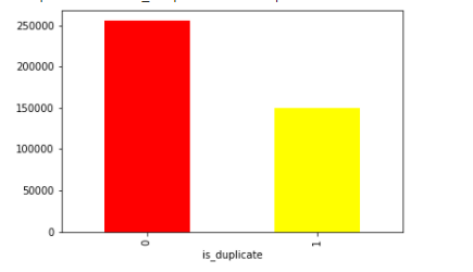
This dataset has 404290 samples with the following features. We aim to predict if two questions are duplicate of each other or not.
[‘id’, ‘qid1’, ‘qid2’, ‘question1’, ‘question2’, ‘is_duplicate’]
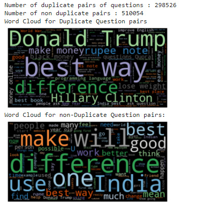
By visualizing the bar plot of distribution of questions, we observe they are balanced.
Wordcloud for similar and dissimilar questions
Similarity model
We have used the following distance calculation functions to compute how similar two sentences are.
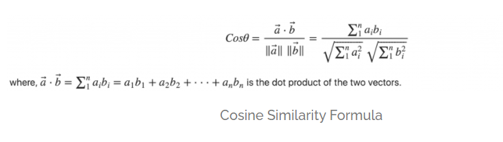
- Cosine Distance
Cosine similarity metric measures the similarity of documents irrespective of their size. Mathematically, it measures the cosine of the angle between two vectors projected in a multi-dimensional space. The uniqueness of the approach if the two similar documents are far apart by the Euclidean distance (due to the document size),they may still be oriented closer together. The smaller the angle, higher the cosine similarity.
- Euclidean Distance Euclidean distance between two points in Euclidean space is the length of a line segment between the two points. The distance between two documents’ words are calculated. One drawback of Euclidean distance is the lack of orientation considered in the calculation — it is based solely on magnitude.

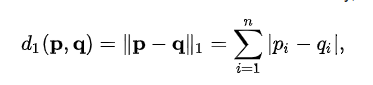
- Manhattan Distance
Manhattan distance is calculated as the sum of the absolute differences between the two vectors. It might make sense to calculate Manhattan distance instead of Euclidean distance for two vectors in an integer feature space.
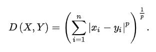
- Minkowski Distance
It is a generalization of the Euclidean and Manhattan distance measures and adds a parameter, p, that allows different distance measures to be calculated. When p is set to 1, the calculation is the same as the Manhattan distance. When p is set to 2, it is the same as the Euclidean distance.
It is common to use Minkowski distance when implementing a machine learning algorithm that uses distance measures as it gives control over the type of distance measure used for real-valued vectors via a hyperparameter “p” that can be tuned.
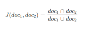
- Jaccard Distance
Jaccard Similarity is also known as the Jaccard index and Intersection over Union. Jaccard Similarity matric measures similarity between two text document based on how the two text documents are in proximity of each other based on the context. Jaccard Similarity defined as an intersection of two documents divided by the union of that two documents that refer to the number of common words over a total number of words. Here, we will use the set of words to find the intersection and union of the document.
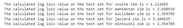
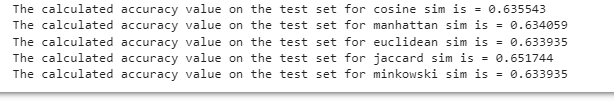
We will use log loss formula to set a base criteria as to what accuracy our algorithm is able to achieve in terms of log loss . We have also computed the accuracy for the distance measures. We set the threshold as 0.5 and if the distance is predicted to be > 0.5, we predict the questions are similar or label 1. If the distance is less than 0.5, we predict the questions are not similar / label 0 So using this metric, we calculated the accuracy for the predictions using these distance metrics.
The logloss output for the training dataset.
The accuracy output for the training dataset.
Clustering Models:
Clustering is an unsupervised Machine Learning Technique. The true labels of the data points are not known and only the data point’s attributes are known to the clustering model. Clustering is the grouping of data points that are similar together into one cluster. This categorization is done on the datapoint’s similarities and differences. The intracluster distances are small and the intercluster distances are large. Some clustering algorithms are DBScan and GMM. Here, we use clustering to determine whether two questions are similar to each other or not.
GMM:
Gaussian Mixture Model is an unsupervised Machine Learning Technique. It is a clustering method. GMM performs soft assignments, unlike K-Means. It is a generative model. It predicts a probability of a data point existing in a cluster instead of a definitive class. GMM is a function that encompasses several Gaussian distributions which are indicative of the number of clusters in the dataset. GMM has three parameters which are the mean, covariance, and the mixing probability. GMM is an expectation-Maximization algorithm. It has an expectation step and a maximization step. In the expectation step, GMM evaluates the responsibilities and in the maximization step, GMM re-estimates the three parameters using the responsibility calculated in the expectation step. GMM can work well on data with varying variances. It is simple to implement.
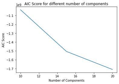
There aren’t great ways to assess and evaluate unsupervised learning methods like clustering algorithms. The key to clustering algorithms is to balance between using too many clusters to divide the data points and using too few clusters to divide the data points. If too many clusters exist, then the variability peaks. One of the parameters for a GMM algorithm is the number of components otherwise called the number of Gaussian distributions. We observed the change in AIC scores for different number of components. As the number of components increased from 10 to 15 to 20, the AIC scores dropped. AIC is the Akaike Information Criteria for a given model. It is a comparative score that estimates the likelihood of a given model giving better results than the other models. Thus, with 20 components, the least score was achieved. GMM is one of the better clustering algorithms. It is appropriate for all covariance types namely full, tied, diagonal, and spherical. GMM is not harsh with its cluster assignments and rather outputs a probability of a data point belonging to each cluster. GMM algorithm is relatively straightforward and simple.
DBSCAN and Variants:
DBSCAN:
DBSCAN is a density-based algorithm. It doesn’t require that every point be assigned to a cluster but instead leaves sparse background classified as ‘noise.’ If the data has variable density clusters, then DBSCAN is either going to miss them, split them up, or lump some of them together based on Hyperparameters. HDBSCAN is basically a DBSCAN implementation for varying epsilon values. The advantage of HDBSCAN is that it allows clusters of varying densities. In DBSCAN, to predict the cluster which the new data points belongs to, we ran through core points and assigned to the cluster of the closest core point that is within eps of the new point. HDBSCAN, provides a function approximate_predict to get the clusters for new data points.
Supervised Machine Learning Methods
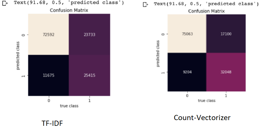
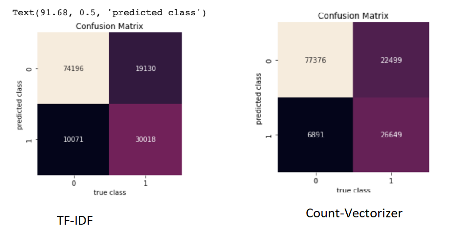
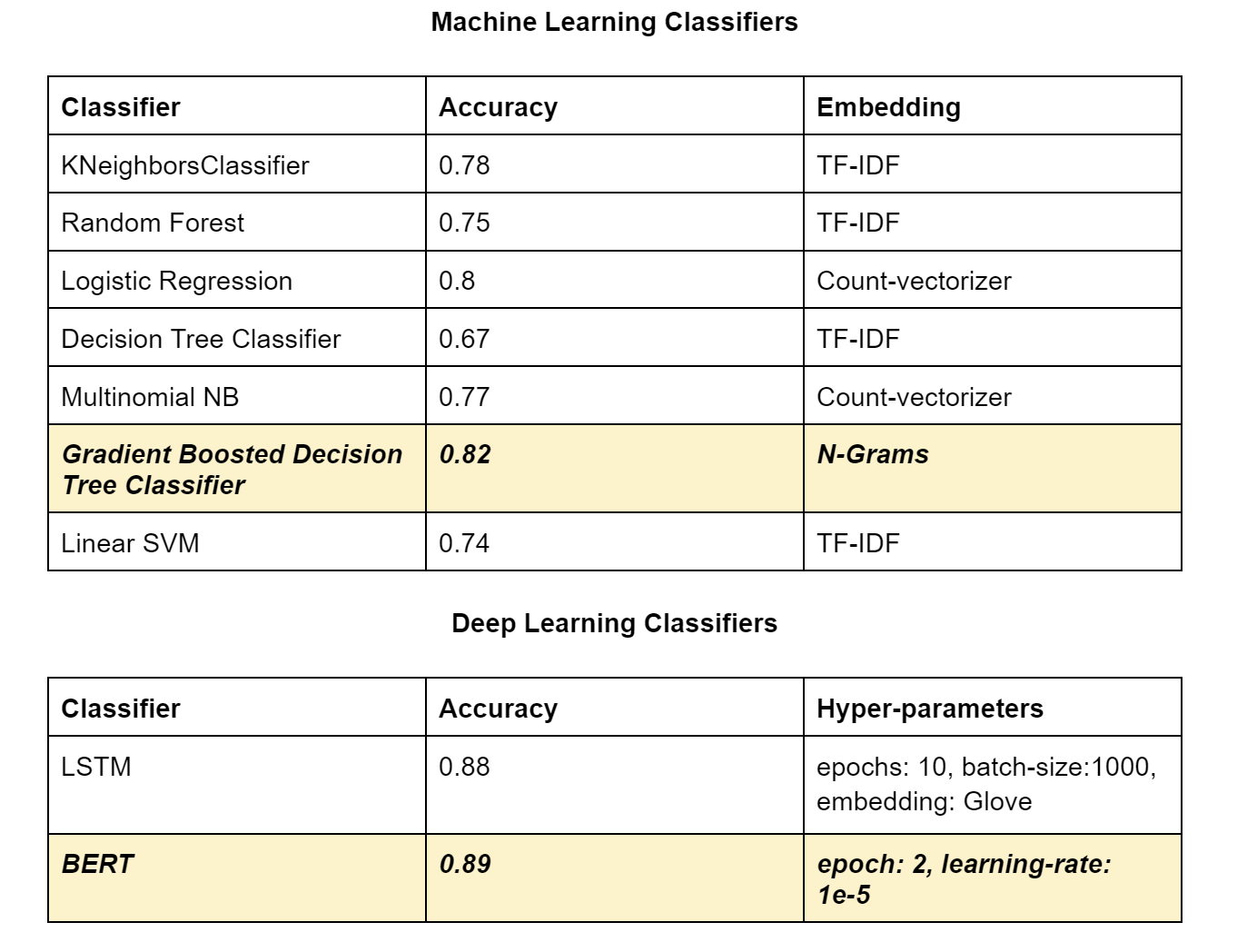
Here we explored Machine Learning models for Question Pairs and created an accuracy table for each model for two different Feature Engineering techniques TF-IDF and Countvectorizer. We used 7 ML models in total: KNeighborsClassifier, Random Forest, LogisticRegression, DecisionTreeClassifier, Multinomial NB, Linear SVM, and Gradient Boosted Decision Tree Classifier. We did hyperparameter tuning for KNeighborsClassifier, Random Forest, Linear SVM and Gradient Boosted Decision Tree Classifier.
Analysis of Features in Question Pair DataSet
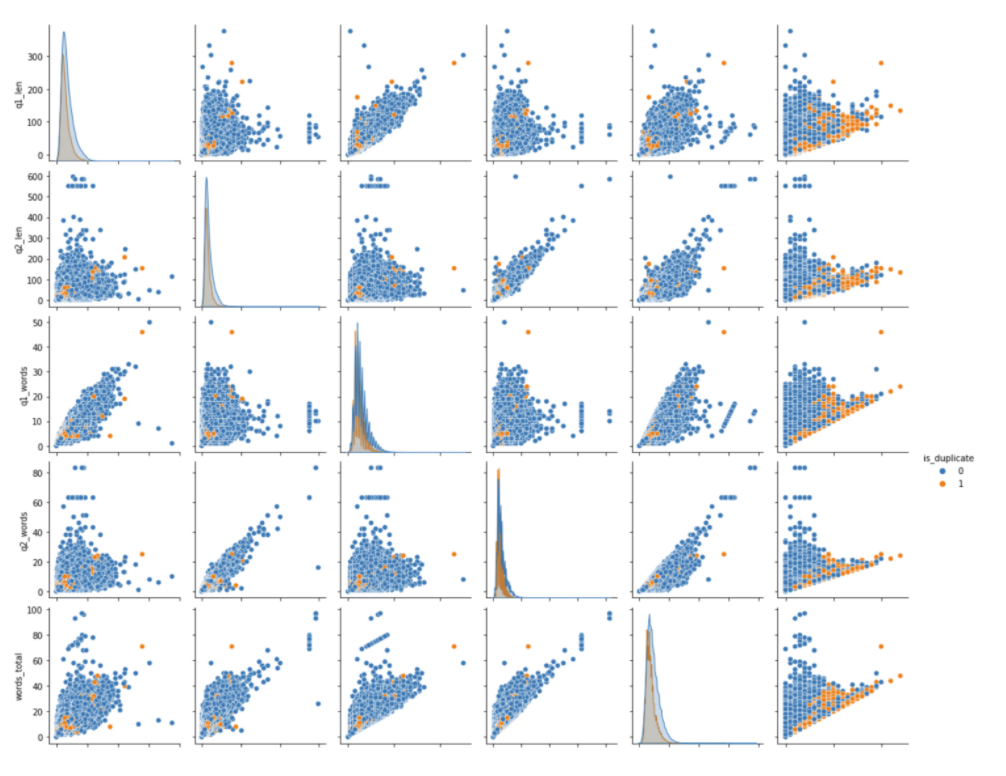
We worked with some of the features like:
Q1_len - question1 length Q2_len - question2 length Q1_words - words in Q1 Q2_words - words in Q2 as well as other derived features like Words_common, last_word_eq (if the last word is equal or not in both the questions), first_word_eq, words_shared (shared words), num_common_adj(common adjacent words), common Part-of-speech (POS) features, etc.
Pair plots for above features
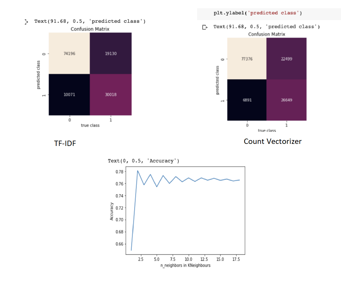
K Neighbors Classifier
We tuned the model until the number of neighbors=20. The classifier gave good results for k=3 and k=4. The graph converges beyond a point with no improvement in performance.
Multinomial Naive Bayes
This algorithm works very well for data that can easily be turned into counts, such as word counts in text. Therefore we decided to use Multinomial Naive Bayes:
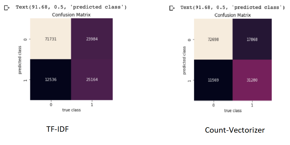
Results Discussion: It works better when using the count-vectorizer for generating the embeddings as it uses the most basic ways to represent text data numerically which always works better when using the Multinomial Naive Bayes classifier.
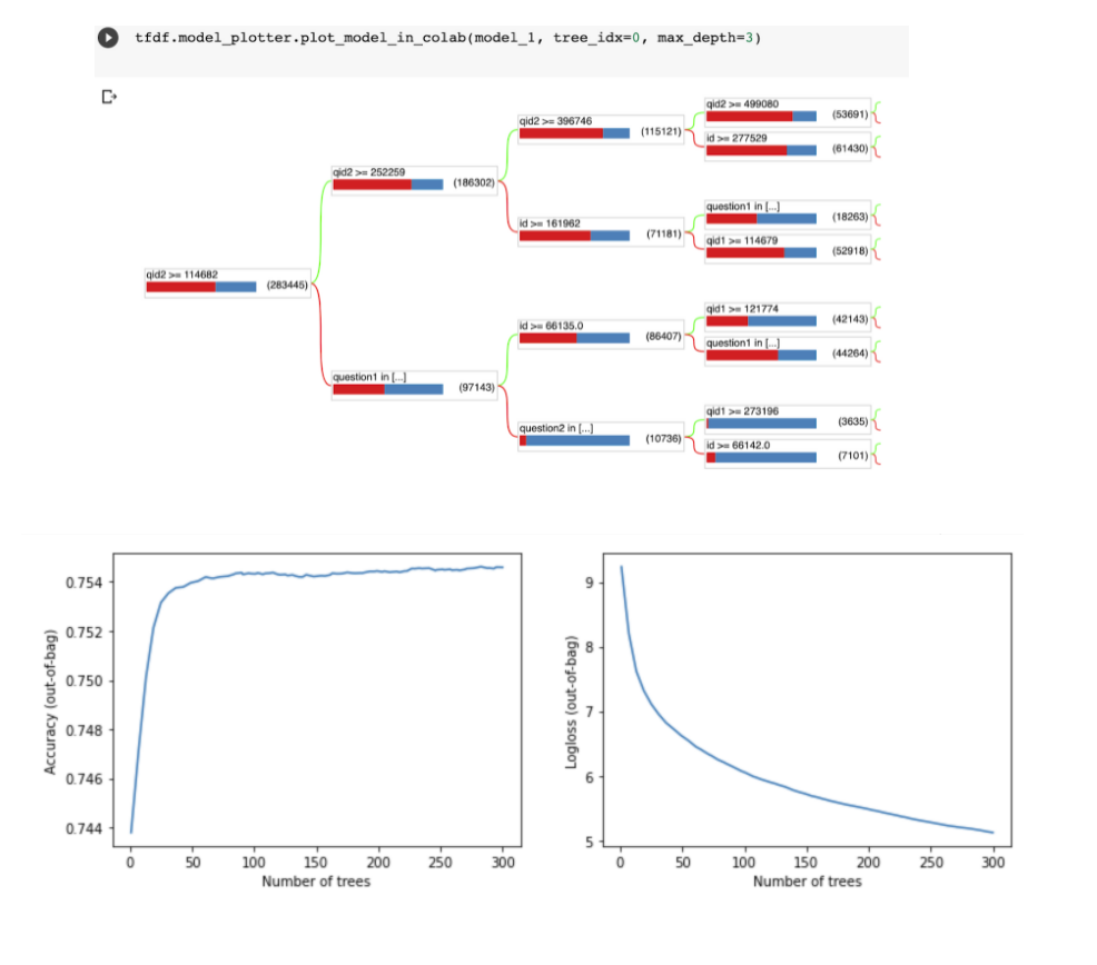
Random Forest
The key point about this algorithm is that it is robust to overfitting, even in extreme cases when there are more features than training data. We used tfdf.Keras.RandomForestModel for training it and performed hyperparameter tuning on the number of trees.
As shown in the graph below, accuracy becomes almost constant after a certain number of trees. The best accuracy obtained is 0.754.
Logistic Regression
The algorithm finds the appropriate weight vector using the questions and tells if they are similar or not.
Decision Tree
Linear SVM
XGBoost
Supervised Deep Learning Methods
LSTM model:
LSTM models are used in this task also to predict similarity. Initially we trained an LSTM model with the Word2Vec Embeddings. For the training metrics, we used accuracy as the classes are fairly balanced.
Word2Vec Embeddings:
Produces Vector representation of the particular word. The word2vec technique uses a neural network model to learn word associations from a large corpus of text data. Word2vec takes into input a text corpus and processes it with a two-layer neural net and outputs a set of vectors. The trained model produces an accuracy of 0.82.
Glove Embeddings :
In an attempt to improve the training accuracy, we used Glove Embeddings to create the feature vector of the questions and use it to train the LSTM. GloVe (Global Vectors) is a word embedding model for distributed representations. It is an unsupervised learning method to get vector representation for words. Words are mapped into meaningful space where the distance between the words is related to semantic similarity. The embeddings are calculated on a globally aggregated corpus and the output vectors demonstrate the linear substructures of the word vector space.
Accuracy was 0.8351
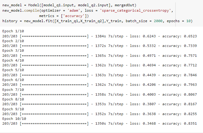
The accuracy vs epoch for hyperparameter batch size = 2000
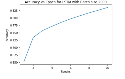
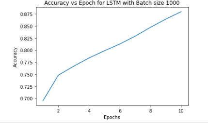
To explore changing hyperparameter’s effect on the accuracy we decided to change the batch size to 1000. This hyperparameter defines the number of data points to evaluate before the internal parameters of the model are updated. Large sizes make large gradient steps compared to smaller ones for the same number of samples “seen”.
On changing batch size to 1000, we found the accuracy improved to 0.8799 at the end of 10 epochs.
The accuracy vs epoch for hyperparameter batch size = 1000
 **
**
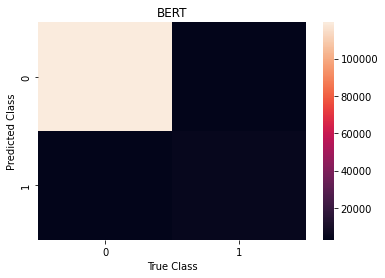
BERT model:
The BERT model has been explained in the previous task of insincerity prediction. For this task, we fine-tuned a BERT model that takes two questions as inputs and that outputs a similarity score for these two sentences. Training is done only for the top layers to perform “feature extraction”, which will allow the model to use the representations of the pre-trained model.
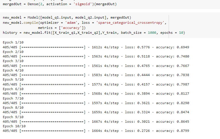
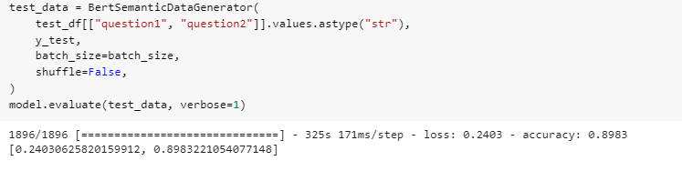
Training is done on the top layers to perform “feature extraction”, enabling the model to use the representations of the pre-trained model. We then trained the data to convergence. Now the fine-tuning step is performed. BERT model is unfrozen and retrained with a very low learning rate. This can deliver good improvement by incrementally adapting the pretrained features to the new data. The final training accuracy is shown in the below image and is 0.9086 after two epochs.
The accuracy of the BERT model on the Test dataset was astonishingly high - 0.8983.
We could see some sample outputs of the BERT model based on the input questions entered.
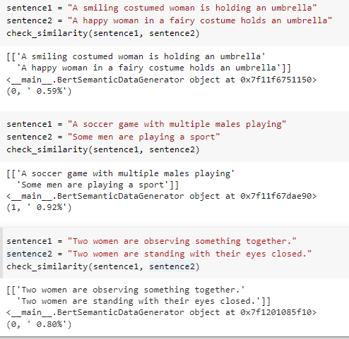
We get a similarity probability and a prediction too.
RESULTS AND DISCUSSIONS
We discuss the approaches we took and summarize our results in the following section.
Results on Quora Insincere Questions Classification Datasets
We started by performing exploratory data analysis on the Quora Insincere Questions Dataset. We observed a huge imbalance in that the number of insincere questions was very less. We used common Natural Language data preprocessing techniques like converting data to lower case text, punctuations removal, stopword removal, Tokenization, Lemmatization to generate features. We also performed feature engineering methods to improve the quality of features. We used Bag of Words, Count Vectorizer, TF IDF vectorization methods in our models and have compared the results in the table. To visualize the words trend, we used Word cloud for visual interpretation and also performed an unsupervised learning method of clustering to get quick insights from the data. To learn more interesting patterns which could be useful for the similar question prediction task as well, we attempted LDA / Latent Dirichlet Allocation, a probabilistic topic modeling technique. We explored the distribution of words for various topic sizes of 10,15,30. We also used LSA / Latent Semantic Analysis for dimensionality reduction on the features. After these steps, we move on to supervised learning methods to compute the predictions. We use the Metrics of Accuracy, F1 score, Precision, and Recall, as our dataset is highly imbalanced and accuracy alone is not enough. We trained models of Naive Bayes, both using TFIDF and Count Vectorizer to compare their performance and plotted confusion matrix of the same. Surprisingly count vectorizer performed better in this case. Then we performed a logistic regression model as it is a binary prediction task on both count vectorizer and TF-IDF. In this case, too, the count vectorizer performed better with a higher F1 score for the insincere class. Moving on to random forests an ensemble method, we observed the same trend of higher F1 scores with Count Vectorizer. Out of all the Machine Leaning models, naive Bayes seems to have the highest performance for the insincere questions. We think it could be because insincere questions usually contain certain bad words which are flagged by the Naive Bayes model ( as it is independent of other features).
Moving on to deep learning models, which we expect to give much better results considering that we have a huge dataset. We start out with Bi-directional Sequence to Sequence Models - RNN, LSTM, and GRU along with pre-trained word embedding like GloVe short form for Global Vectors for word representation, Wiki News FastText embeddings, and Paragram embeddings. We have compared the accuracy and F1 score of these models against each other and found Bi-LSTM to be the best performer among the three for all types of word embeddings. However, using BERT, a transformer model, it outperforms them all with a higher F1 score. BERT comes with its own embeddings.
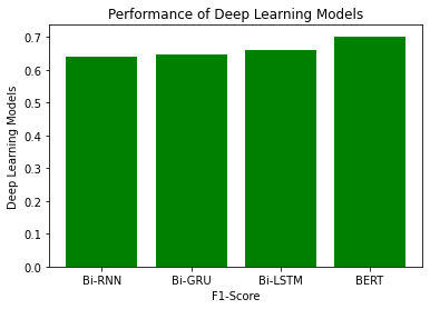
The best embedding results of each model are displayed in the below table.
Results on Quora Question Pairs Dataset
We did exploratory data analysis to observe the occurrence of common words and distribution of data and found it to be balanced. Hence we decided to use Accuracy Metric for training models. To compute the semantic similarity between two questions, we initially started with the distance models Cosine Distance, Euclidean Distance, Manhattan Distance, Jaccard Distance, and Minkowski distance. We obtained the best accuracy for the Jaccard metric which is 0.651.
We trained multiple Machine Learning models with multiple to predict if two questions are similar or not. We observed that both embeddings of TF-IDF and Count Vectorizer provide good accuracies with ML Models. KNN and Random Forest and Multinomial Naive Bayes have a comparable accuracy around 0.75 - 0.78. Linear SVM has good accuracy and Decision Tree Classifier has lower accuracies. Gradient Boosted Decision Tree Classifier is the best model with an accuracy of 0.82 .
Deep Learning model LSTM - with Word2vec and Glove tuned for different batch sizes hyperparameter was trained. Similarly, the BERT model was trained ( on the last few layers) with a learning rate of 1e-05 and obtained the best accuracy of 0.9086 on the training dataset.
For the task of finding the top 5 similar questions, we use Gaussian Mixture Models Clustering. After feature engineering to get 300 features ( the maximum amount memory could handle) using TF-IDF, we performed GMM multiple times with input components increased from 10 to 20 in increments of 2. The best AIC score ( lowest in value) was observed for 20 components and we fixed that for our final model. As GMM is a soft clustering method, we used this to determine similar questions.
While further work can improve performance, we believe our models perform to good accuracies on both these tasks.
Showcasing the output of our local site when user enters two questions as input. We predict if they are similar.

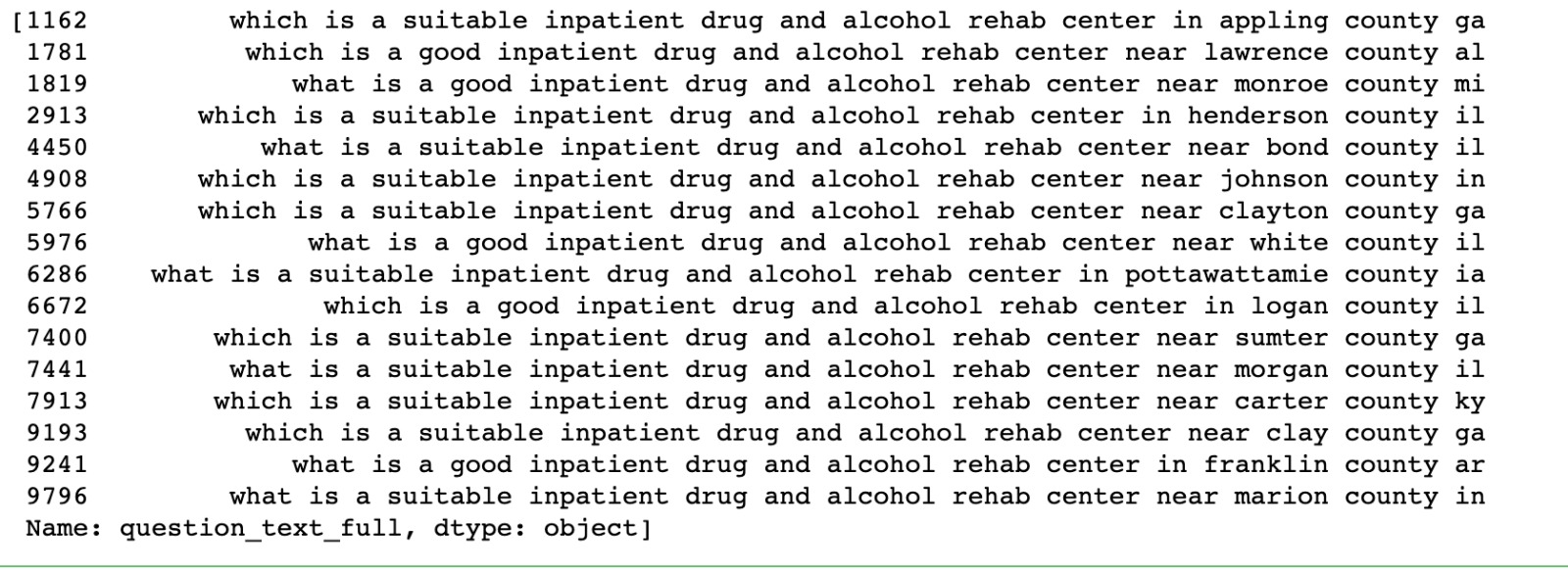
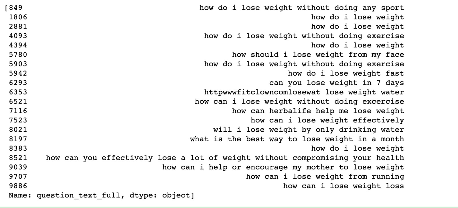
Showcasing the output of our local site when user enters one questions as input. It also outputs similar questions from the dataset.

CONCLUSIONS
In our project, we worked on solving the major problems faced by the popular question and answer site Quora. We set out with an ambitious goal to perform the following tasks -
- classify if a question is insincere or not,
- predict if two questions are similar and
- given a question display the most similar questions present in the question corpus.
We worked on the two datasets - Quora Question Pairs and Quora Insincere Classification for these tasks and we learned a lot along the way. We explored a lot of techniques in the areas of Natural Language Processing, Machine Learning - Supervised and Unsupervised, Topic Modelling, Clustering, and Dimensionality Reduction. We also worked on the state-of-the-art Deep Learning models and tried various text embedding methods to obtain the best accuracies and F1 scores. We developed a local StreamLit App in which we have the results of our best models to perform the required query. We have completed all the Proposed Objectives we stated at the start of the semester and produced the above results.
CONTRIBUTION
All team members contributed equally to the project.
References
- [1810.10641] Predicting the Semantic Textual Similarity with Siamese CNN and LSTM
- [1807.02854] Replicated Siamese LSTM in Ticketing System for Similarity Learning and Retrieval in Asymmetric Texts
- Text Similarity with Siamese Recurrent Networks
- Proceedings of the 24th ACM International on Conference on Information and Knowledge Management: Short Text Similarity with Word
- A Survey of Text Similarity Approaches
- https://en.wikipedia.org/wiki/Word2vec
- https://colah.github.io/posts/2015-08-Understanding-LSTMs/